Trends in Petroleum Engineering

Causes of oil price increase have been a subject of much interest and numerous studies given the importance of oil as the main source of energy of the world. In the last two decades, the price volatility of crude oil has always remained a controversy. Literature has two views. The first view argues that the changes in oil prices are due to supply and demand. The other claims that financial variables (speculation and futures markets) are vital in crude oil price changes. The advent of new variables that serve as paradigm for oil price volatility creates the need to understand the intricacies of the oil market. This paper investigated the factors that determine the prices of crude oil together with the degree to which prices have been affected by the global health pandemic the Corona Virus Disease (COVID-19) in 2020 by employing a multiple regression method in its assessment. With oil price as the dependent variable, all other variables were analyzed to assess the dependency of the crude oil prices on these independent variables. Refinery capacity, Organization of Petroleum Exporting Countries (OPEC) production and oil trade movements were found to be the main affecting factors in this work whilst the cases and deaths arising from the COVID-19 confirmed cases and recorded deaths in the year 2020 proved insignificant as a determining crude oil factor.

Keywords: Oil price, Corona Virus Disease (Covid-19), Multiple regression, Refinery capacity, OPEC (Organization of Petroleum Exporting Countries) production and Oil trade movement

Crude oil has undeniably been a remarkable source of nonrenewable resource in the last two centuries. Crude oil is essential in the production of energy and used in the manufacturing, domestic, medicinal, transportation, and economic sectors. It also is a frontline requirement in today's hydrocarbon society. Oil remained the world's leading fuel, accounting for 33% of global energy consumption, according to the BP statistical analysis of world energy 2020.¹

Following Colonel Edwin Drake's successful drilling of the first oil well at Oil Creek near Titusville in West Pennsylvania in 1859, the crude oil market started in the 1860s. Western Pennsylvania's early production grew quickly, from around 450000 barrels in 1860 to 3 million barrels in 1862. Demand quickly outstripped supply, and by the end of 1862, prices had risen to $4 a barrel, and by September 1863, prices were soared to $7.25 a barrel.²

Crude oil's economic uncertainty is due to its ever-increasing demand and emergence as a highly sought-after global commodity. The Organisation of Petroleum Exporting Countries (OPEC), speculators, and major oil firms have all been recognized as determinants of crude oil prices across various participants in the public debate. It also turned out that crude oil prices react to other variables such as economic news, overall supplies as a result of increasing demand driven by economic and industrial growth, geopolitical and economic events, net importing oil countries, the value of the dollar, weather and natural disasters.³

Crude oil is used in almost every aspect of modern life, it is critical to recognize and comprehend the factors that influence its pricing in the modern era, which is being impacted by a worldwide threat-the COVID 19 pandemic. In 2020, the coronavirus pandemic led to a significant fall in crude oil prices, as seen in the response of prices to global changes during the Oil Wars and the major oil crisis of 1973/1974.

The goal of this paper is to determine crude oil price determinants and the impact of COVID-19 on crude oil prices in 2020.

Modelling software

The JMP statistical software was employed to generate a regression model between oil price and its determinants and also the impact of COVID-19 on oil prices in 2020. JMP statistical software was launched in 1989 and is very useful in statistical interactivity and forms the core basis of accuracy, value and quality whilst providing a wide range of computation and graphical applications.

Data acquisition

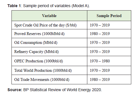
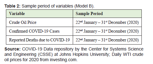
The BP Statistical Review of World Energy 2020 worksheet provided secondary data on several of the factors. Also, data for the daily reported cases and confirmed deaths due to the coronavirus spanning the year 2020 was collected from the COVID-19 Data Repository by the Center for Systems Science and Engineering (CSSE) at Johns Hopkins University whilst daily WTI crude oil prices for 2020 was sourced from investing.com. Tables 1 and 2 show the sample period of the data collected and its units for model A and B respectively. For full data used see Appendixes A and B.

Regression analysis

A Multiple regression using Standard Least Squares method was employed with oil price as the dependent variable and the other variables shown as independent variables. Least square approach is used to determine a line of best fit by minimizing the sum of squares created by a mathematical function. A “square” is determined by squaring the distance between a data point and the regression line. This approach limits the distance between a function and the data points that a function is trying to explain.⁴

Dependent variable

The dependent (response) variable is global crude oil price. The prices represent the average annual money of the day prices of Arabian Light posted as Ras Tanura from 1970-1983 and Brent dated from 1984-2019, traded in U.S dollars per barrel ($/bbl) and the average daily money of the day prices of Brent crude from 22^nd January 2020 to 31^st December, 2020 with all denoted as p_i.

Independent variables

The independent variables of the regression equation are.

1. i. Proved Reserves: The estimates in this table have been compiled using a combination of primary official sources, third-party data from the OPEC Secretariat, World Oil, Oil & Gas Journal and Chinese reserves based on official data and information in the public domain. Canadian oil sands ‘under active development’ are an official estimate. Venezuelan Orinoco Belt reserves are based on the OPEC Secretariat and government announcements. Reserves and R/P ratio for Canada includes Canadian oil sands. Reserves and R/P ratio for Venezuela includes the Orinoco Belt. Saudi Arabia’s oil reserves include NGLs from 2017. Reserves include gas condensate and natural gas liquids (NGLs) as well as crude oil. Shares of total and R/P ratios are calculated using thousand million barrels figures.⁵
2. ii. Oil Consumption: Data includes inland demand plus international aviation and marine bunkers and refinery fuel and loss. Consumption of bio gasoline (such as ethanol), biodiesel and derivatives of coal and natural gas are also included and measured in thousand barrels per day.
3. iii. Refinery Capacity: To evaluate the effects of the refinery sector on crude oil prices, data was collected on refinery capacity measured in a thousand barrels per day.
4. iv. OPEC Production: OPEC’s influence is measured by production rates from its member countries. Denoted as (opd) in units of a thousand barrels of oil per day (Mbbl/d).
5. v. Oil Production: The global yearly production of crude oil measured in a thousand barrels per day includes crude oil, shale oil, oil sands, condensates (lease condensate or gas condensates that require further refining) and NGLs (natural gas liquids-ethane, LPG and naphtha separated from the production of natural gas). It excludes liquid fuels from other sources such as biofuels and synthetic derivatives of coal and natural gas. This also excludes liquid fuel adjustment factors such as refinery processing gain. It also excludes oil shales/kerogen extracted in solid form.
6. vi. Oil Trade Movements: The global yearly data for oil trade movements exclude the intra-area movements of oil (for example, crude oil and products moving between countries within Europe). They do not include biofuels. Bunkers fuel is not included as exports. Crude imports and exports include condensates. Saudi Arabian exports from 1980 are also available in the oil trade movements denoted in million tonnes and thousand barrels per day.

Confirmed COVID-19 Cases: Raw data on confirmed cases for all countries is sourced from the COVID-19 Data Repository by the Centre for Systems Science and Engineering (CSSE) at Johns Hopkins University.

Reported Deaths due to COVID-19: Raw data on reported deaths for all countries is sourced from the COVID-19 Data Repository by the Centre for Systems Science and Engineering (CSSE) at Johns Hopkins University.

Model Specification

The normal multiple regression model specification is given as follows.

p_i=α+β₁X₁+β₂X₂+β₃X₃+e_i (2.1)

take

p_i= dependent variable

α= intercept

X_i= independent variable

β= unknown parameters

e_i= error terms

Hypotheses

The analysis of this work was done based on the following hypotheses: where;

H₁: presents the research hypothesis; and

H₀: the null hypothesis.

Model selection criteria

Several models with different combinations of independent variables were run to generate the most appropriate and efficient model. The selection of the most appropriate method was based on the following limitations and goodness of fit statistics associated with multiple regression.

Limitations of multiple regression

Some limitations of multiple regression include:

1. i. Overfitting: Adding more independent variables to a multiple regression procedure does not mean the regression will be better or offer better predictions. It can lead to worse situations and this is called overfitting (Ray, 2015).
2. ii. Multicollinearity: Multiple regression requires that the model generated possess no or very little multicollinearity. This phenomenon occurs when the independent variables are not only potentially related to the dependent variable but are also potentially related to each other (Ray, 2015). Variables that are highly correlated were not combined in the same model in order to reduce redundancy and unstable coefficient estimates caused by multicollinearity.

Goodness of fit statistics

The following statistical characteristics were considered in selecting the right model:

1. i. F Test: It compares a model with no predictors (intercept-only model) to the model specified. The hypotheses for the F-Test of the overall significance are as follows:
2. ii. H0: The fit of the intercept-only model and your model are equal.
3. iii. H1: The fit of the intercept-only model is significantly reduced compared to your model.
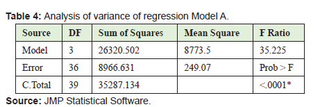
4. iv. If the P value for the F-test of overall significance test is less than most commonly used significance level (0.05), the null hypothesis can be rejected and it can be concluded that the model generated provides a better fit than the intercept-only model.
5. v. T Test: This test compares the data of a variable to its null hypothesis by generating a t value. If the probability (p-value) of the t value falling within the rejection region of a T distribution is fairly low, the null hypothesis can be rejected using the common significance level of 0.05. Thus, a low p-value (< 0.05) indicates the predictor variable has a meaningful impact on the response variable.⁶
6. vi. Standard Error of Regression (S): This statistic provides an overall measure of how well the model fits the data. It represents the average distance that the observed values fall from the regression line. Conveniently, it tells you how wrong the regression model is on average using the units of the response variable. Smaller values are better because it indicates that the observations are closer to the fitted line.⁶
7. vii. R Squared: It measures closeness of the fitted regression line. It is the percentage of the response variable variation that is explained by a linear model.
8. Viii. Generally, a higher R-squared, implies a better model fit. It is always between 0 and 100%.⁶
9. ix. R Squared Adjusted: The adjusted R-squared compares the explanatory power of regression models that contain different numbers of predictors in the model. The adjusted R-squared increases only if the new term improves the model more than would be expected by chance. It decreases when a predictor improves the model by less than expected by chance. It is always lower than the R-squared.⁶

Regression Model

Regression Model A

The parameters that proved important in the regression model for the independent variables in dataset A, include refinery capacity, OPEC production and oil trade movements. All other independent variables constituted a percentage of 0.6% in the total regression model and could hence be flagged insignificant.

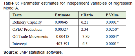
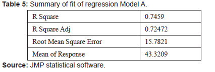
Table 3, 4 and 5 below shows the Parameter Estimates, Analysis of Variance and the Summary of Fit for the independent variables in dataset A as sourced from Data Inputs in the statistical tool, JMP.

Regression Model A Equation is given as follows:

p__i=-403.5912+0.0065(Refinery Capacity)+0.0033(OPEC production)-0.0042(Oil trade movements). (3.1)

Regression Model B

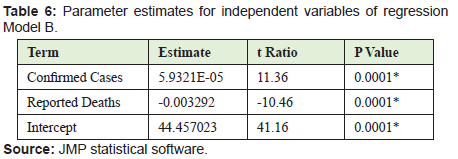
The tables below shows the Parameter Estimates, Analysis of Variance and the Summary of Fit for the independent variables in dataset A Tables 6-8.

Regression Model B Equation is also given as follows.
p__i=44.457023+5.9321e-5(COVID-19 cases)-0.003292(COVID-19 deaths) (3.2)

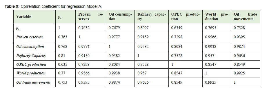
Tables 10 show the Pearson’s correlation coefficient (R coefficient) for Regression Model A and B respectively.

Analysis of Results

Regression models

The first regression model constitutes of refinery capacity, OPEC production and oil trade movements as the most significant independent variables. With an R-squared (R²) adjusted value 0.725, it means that 72.5% of the increase or changes in crude oil prices is due to changes in the significant independent variables stated in equation 4.1.

Regression model B explains the impact of COVID-19 confirmed cases and reported deaths on the price fluctuations in the year 2020. From the analysis of data in Table 5, confirmed cases and reported deaths arising from the corona virus disease caused 34.9% in the fluctuations that occurred in the crude oil prices. This can be seen in an R-squared (R²) adjusted value of 0.3487.

Refinery capacity

At a 1% significance level, refinery capacity is confirmed as a significant determinant of crude oil prices. With a coefficient of 0.0065, it indicates that an increase in crude refinery utilization rates by 1% leads to an average increase in oil prices by 0.0065% all other factors held constant. Also, the Log-Worth for refinery capacity reads at 6.432 rendering it significant at the 0.01 level.

From theory, high refinery utilization rates can be taken as a sign of shortages in the supply of petroleum products7 which will increase prices on petroleum products, such as gasoline and again increase crude oil prices. Also, the relationship can be negative. High utilization rates might indicate that too much petroleum products are flowing into the market, causing prices to decrease. Refinery utilization rates thus have both a positive and negative relationship with crude oil prices.

The relationship between refinery capacities and prices is explained using a trend analysis shown in Figure 1.

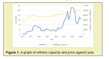
The trend of refinery capacity shows quite a sharp increase in earlier years followed by a gently downward movement and a steady, stable increase. The trend of price shows a general upward movement with a lot of fluctuations and instability within the years studied. The two trends are not identical as one is fairly stable and the other highly volatile. Although both trends tend to increase towards current years, there is no significant or concrete movement in refinery capacity’s graph that can be attributed to the fluctuations in prices. Thus, although refinery capacity rates play a role in pricing, its relationships with prices in the inverse or positive direction cannot be determined from this graph.

Olimb and Ødegård in 2010, established both negative and positive relationship of refinery capacity rates with oil prices using a time varying approach. Möbert (2007) found a positive relationship, while Kaufman et al., in 2005 found a negative relationship.⁸

OPEC Production

OPEC’s production has been statistically proven as a vital contributor in the determination of oil prices. With a corresponding t-ratio of 2.34 it further states categorically the evidence that OPEC production is against the null hypothesis.

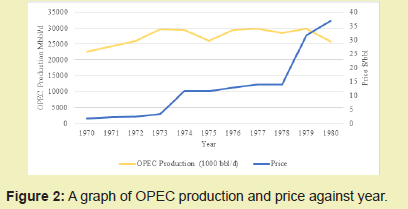
Figure 2 monitors OPEC’s impact on prices during the 1970’s where it held its highest market dominance. OPEC’s gradual plateau and decrease in production from 1972 to 1975 caused a sharp spike in oil prices. Prices became fairly stable when production rates began to increase after 1975 and the sharp price increase from 1979 responded to declining production rates from 1977.

Oil trade movements

Oil trade movements generally represent the oil market for producers and consumers. From the Spearman’s correlation coefficient, there is a correlation of 0.99 between oil trade movements with oil production and oil consumption. The regression model indicates a coefficient of -0.00418. This means an average increase or decrease of 1% in oil trade movements will cause 0.00418% decrease or increase in oil prices.

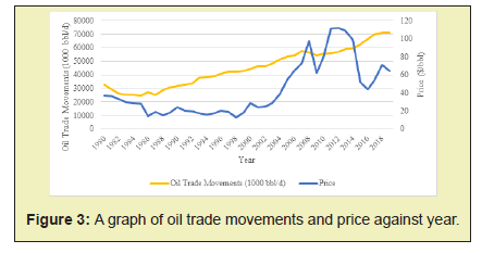
In Figure 3 oil trade movements in the early years after the oil crisis in 1970’s showed a gradual decrease in both trade movements and oil prices from 1980 to 1985. After this, a sharp increase in movements in the following years saw a steep fall in oil prices. At the tail of the graph, prices can be seen slightly rising above oil trade movements due to subsequent falls experienced in oil trade movements. The graph can be said to support the statistical hypothesis of an inverse relationship between oil trade movements and oil prices.

2020 Crude oil graph

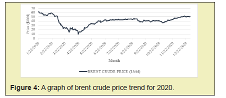
During the first half of 2020, market uncertainties persisted for all energy sources as shown in Figure 4. High levels of inventory forced Brent crude oil spot prices down from a monthly average of $64 per barrel in January to only $9 a barrel in April. As the year went on, oil markets started to shift as nations began to emerge from lockdown. The month of June saw Brent crude oil spot prices average $40 per barrel, an increase of $11 per barrel from May’s average. Production cuts by OPEC and their partner counties contributed to the stabilization of oil prices. Oil prices continued their rebound from April lows as the year progressed synonymous to market expectation growths. Optimism about the possible rollout of multiple COVID-19 vaccines also buoyed the market. In November, Brent crude oil spot prices increased to an average of $43 per barrel, an increase of $3 a barrel from October’s per barrel average.

Confirmed COVID-19 cases

The data for daily confirmed cases as a result of exponential infection rates gave an output of 0.000059 coefficient in Regression Model B. Figure 5 is against the null hypothesis stating that confirmed COVID-19 cases in the year 2020 were a contributing factor in determining the fluctuating prices that occurred with the pandemic.

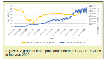
With a correlation and regression coefficient of 0.2395 and 0.000059, confirmed COVID-19 cases could be said to be the more determining factor in the R-squared adjusted value for regression model B. Again Fig. 5 shows how responsive prices were to the early days of the virus with levels reaching as low as $9 in April when there had been an exponential increase in COVID cases. The beginning of the second half of the year saw oil prices to be stable from gradual rise in the preceding months.

Reported deaths due to COVID-19

The regression model shows an inverse relationship of COVID-19 deaths to oil prices. This is supported by a t-ratio of -10.46 which supports the evidence that Reported deaths due to COVID-19 agrees to the null hypothesis of not being a significant factor in oil price determination in the year 2020.

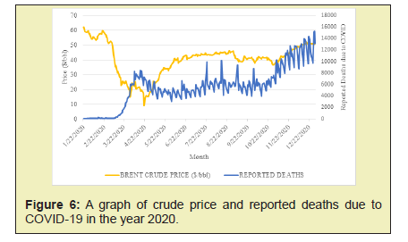
From Figure 6, crude oil prices could be said to have been responsive to deaths arising from infected persons more in the first quarter of the year. This can be interpreted as a global response to the shock the virus arrived with. The following months saw a non-responsive correlation to price changes since prices gradually increased in the middle of the year and further increased more to the end of the year synonymous to COVID-19 deaths. It can be concluded from the regression model and the Spearman’s correlation coefficient that reported deaths due to COVID-19 agrees to the null hypothesis.

Eight different factors were evaluated in this research using regression models and several other factors from literature. Six of these factors made the first regression model which focused on a 49-year period between 1970 and 2019 pre COVID whilst the second regression model took into consideration the effects of confirmed COVID-19 cases and deaths on the already established fluctuating oil prices. The evaluated factors were shown to behave in accordance with the hypotheses of the research. From the analysis of data, it can be concluded that:

1. i. Refinery capacity, OPEC production and global oil trade movements are significant crude oil price determinants.
2. ii. COVID-19 confirmed cases and deaths recorded in the year 2020 contributed insignificantly to the fluctuations that occurred in crude oil price.
3. iii.Crude oil prices change over time and cannot be attributed to one single market factor, or just the explanatory factors analysed in this work.

None.

None.

The authors declare no conflicts of interest regarding the publication of this paper.

1. 1. Anon. “2019 in Review”. BP Statistical Review of World Energy Journal 2020. 69th (edn):pp.1-47.
2. 2. Yergin D. The Prize: The Epic Quest for Oil, Money & Power, Simon & Schuster, New York. 1991:pp. 1-78.
3. 3. King K, Deng A, Metz D. An Economic Analysis of Oil Price Movements: The Role of Political Events and Economic News, Financial Trading and Market Fundamentals”, Bates White Economic Consulting, Washington DC. 2012;pp.1-52.
4. 4. Ray S. 7 Types of Regression Techniques You Should Know! 2015.
5. 5. BP Statistical Review of World Energy June 2020 Workbook. 2020.
6. 6. Frost J. Regression Analysis Tutorial and Examples. The Minitab Blog. 2013.
7. 7. Olimb M, Ødegård TM. Understanding the Factors Behind Crude Oil Price Changes A Time-varying Model Approach. Unpublished MSc Thesis Report, Norwegian University of Science and Technology. 2010;pp.1-45.
8. 8. Mobert J. Crude oil price determinants. Published MSc Thesis Report, Germany Darmstadt Discussion Papers in Economics. 2007;186:pp.32.