Trends in Petroleum Engineering

Heavy oil accounts for a portion of the world's total oil reserves. The volume of heavy oil reserves is double that of normal oil reserves. As conventional oil reserves run out, heavy oil and bitumen have a lot of promise to meet some of the world's future energy needs. The ability to drill horizontally has paved the door for Steam Assisted Gravity Drainage (SAGD). This study sought to investigate the use of machine learning and numerical simulation in assessing the performance of a high viscous reservoir via SAGD process. A reservoir model was built using the CMG software. The model built mimicked high viscous reservoir conditions in 3D. Various simulations were run using the STARS simulator which is used for advanced thermal/chemical process like SAGD. Multivariate Adaptive Regression Splines (MARS) and Treenet gradient boosting machine (Treenet GBM) were used to predict the results from CMG and validate the predictions. The results obtained showed the horizontal well giving a higher oil recovery factor than the vertical well. In addition, the cumulative oil production from the horizontal well were also higher than the vertical well. The predictions from CMG gave a better validation from the MARS (cumulative oil production had R²=0.99758; MAPE=0.01889) as compared to the Treenet GBM (cumulative oil production had R²=0.9010; MAPE=0.02456).

Keywords: Heavy oil, Steam assisted gravity drainage, MARS, Treenet GBM

The world’s total world oil resources may range from 9 to 13 trillion barrels.¹ However, only about 1.7 trillion of these resources may be classified as reserves (British Petroleum, 2017). A large part of the world oil resource, about 70% of total world oil resources (6.3 to 9.1 trillion barrels), exists in the form of heavy oil which can be defined by an API gravity of less than 22 and viscosity of larger than 100 cp. Venezuela and Alberta, Canada, have most of these heavy oils originally in place which can be estimated to be more than 1.8 trillion and 1.7 trillion barrels, respectively. Moreover, Alaska oilfields also contribute to the world heavy oil resource in the range of 20 to 25 billion barrels.² This implies that there is a vast oil reserve lying dormant and not exploited.

Light oil on the other hand accounts for about 30% of the total world oil resources. Until recently, the amount of light oil available met global demand. “According to the 2022 IEA report, oil demand growth increased to 2.3 million barrels per day in 2022 and is projected to rise to 1.7 million barrels per day in 2023”. This shows how conventional oil reserves are depleting at faster rate while the demand and consumption of oil is increasing rapidly. There is therefore the need to turn our attention to unconventional oil resources to meet the demand of the global market.³ Thus, as the supply of light oil diminishes, new sources, such as heavy oil and natural bitumen, must be examined. As a result, heavy oil and other resource recovery play an essential role in the petroleum sector. The viscosity and gravity of heavy oils vary from 100 to 10,000 cp and 20 to 10 API, respectively. Heavy oil is modestly mobile in the reservoir due to its high viscosity and low API, thereby making traditional production techniques difficult to employ. This is due to its high viscosity which makes the flow of the oil difficult.

Additional efforts are therefore needed to guarantee the viability of oil recovery from heavy oil reservoirs.⁴ Among the methods that can be used to improve oil recovery rates from high viscous reservoirs are secondary and tertiary methods, most importantly Enhanced Oil Recovery (EOR) methods. EOR methods such as Steam Assisted Gravity Drainage, which use thermal recovery techniques, rely on the reduction of oil viscosity through the use of heat. This technique is well suited for effectively unlocking heavy oil resources.² With today's improved technology, it is now possible to extract oil from previously unrecoverable or unconventional sources and make lots of profit due to the large increase in oil prices. This study sought to simulate the performance of a high viscous reservoir via the Steam Assisted Gravity Drainage (SAGD) technique.

Steam Assisted Gravity Drainage (SAGD) Process

This process is a thermal recovery technique which involves the injection of steam into subsurface oil sands deposits in order to heat the hydrocarbon resource trapped in the sand, lower mobility ratio by reducing viscosity and/or vapourising part of the oil and cause the oil to flow freely enough to be recovered.^5,6 It is widely used for heavy oil and bitumen recovery. The process is a complex oil displacement method involving simultaneous heat, mass, and fluid transport.⁷ In the process, a pair of horizontal wells are bored into the rock formation (one around 5-10 meters above the other) to retrieve heavy oil from underground pay zones. The schematic of the process is shown in Figure 1. In the process steam is injected through a horizontal well to decrease the viscosity of the heavy oil/ bitumen, allowing it to flow to an adjacent horizontal well. The upper section (top horizontal well) is referred to as a steam injection well (injector) while the lower section (lower horizontal well) is referred to as a production well (producer).

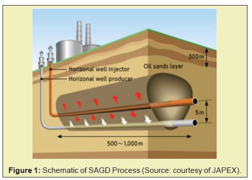
Water is converted to steam, circulated through the top well (injector) and into the oil sand reservoir. The steam subsequently exits the upper well and spreads out in all directions throughout the formation. Heat is transported from the steam to the heavy oil sand thereby reducing the oil viscosity and allow it to flow more easily downward (under gravity) into the production well. Gravity drainage is the term used to describe how the heavy oil drain.⁶ The schematics of a mobilized oil flowing to the horizontal production well under gravity is shown in Figure 2.

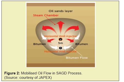
The injected steam reduces the oil viscosity to 1–10 cp depending on reservoir conditions such as temperature and fluid properties of the oil. The most prevalent gases produced during SAGD are methane, carbon dioxide and traces of hydrogen sulphide.⁸ The injected steam runs to the steam chamber's edges and transfers its latent heat to the heavy oil/bitumen in SAGD. This results in heating the oil zone beyond the chamber edge and consequently, the viscosity of heavy oil/bitumen is lowered.⁶

This technology is incredibly efficient, with claims that it can recover 60-70 percent of the oil in place, making it the most efficient thermal enhanced oil recovery method available.⁸ In comparison to other steam-based processes, the SAGD method enhances steam oil ratio in addition to high ultimate recovery. Because there are no pressure-driven instabilities like coning, channelling or fracturing in the SAGD process, it is relatively stable compared to other processes. It is purely a gravity-driven process which is quite stable, and the process zone only grows as gravity segregation occurs. However, in order to have an effective SAGD production, the injected and generated volumes must be balanced as a result of which the volume balance is maintained.⁸

Challenges related to SAGD

In all procedures involving the injection of hot fluid, heat loss from the injection wells to the overburden formations is a concern. A greater proportion of the injected heat is likely to be lost if the injection wells are inadequately insulated and the injection rates are low. This effect may be increased with regard to reservoir depth due to the distance that steam must travel to reach the reservoir. In the case of steam-based technology, this results in steam condensing as a result of the heat loss. As a result, the steam may enter the reservoir as hot water, worsening the effects of hot water flooding. Measures should be made ahead of time to ensure that injection wells are completed in a way that prevents steam condensation.^8,9

The short lifespan of SAGD wells is one of its drawbacks, thus it is critical to make sure that the drilling costs do not outweigh the money gained by production. Another drawback of SAGD is the high cost of steam. In order to maximize the economic outcome, it is critical to keep the steam oil ratio as low as feasible.³

CMG, the pioneer in Enhanced Oil Recovery simulation, was used for simulation as it supplies software that is easier to use and produces the most accurate results for compositional, conventional, unconventional and advanced EOR processes.

Dataset

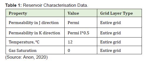
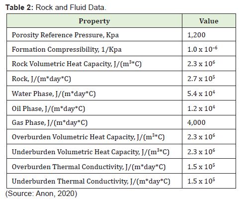
The study's base case data file and initial input data are from work done by CMG in the year 2020. The dataset were characterised into three sections as follows:

1. i. Reservoir Characterisation;
2. ii. Rock and Fluid Properties; and
3. iii. Steam Injection Conditions.

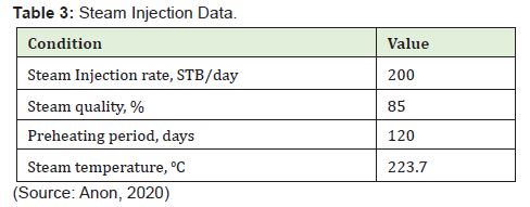
The data for the reservoir characterization, rock and fluid properties and steam injection are presented in Table 1, 2 and 3 respectively.

Reservoir model development

Numerical simulation model was used in the development of the reservoir model. The reservoir model was developed using the following steps:

1. i. A new reservoir model was built using the STARS simulator. This model was based on the reservoir and fluid characteristics (See Table 1 and 2).
2. ii. An injector and a producer well were made into the reservoir to enable the fluid to flow.
3. iii. In order for the oil to flow, steam (heat) was pumped into the injector well to lower the viscosity of the oil.
4. iv. Finally, a commercial simulator was used to validate the created reservoir model using the STARS simulator.

Numerical Model Procedures

The procedures or the steps used in building the base case model are outlined below.
Setting up base case model

The Builder which was used in building the model was launched to create a new model. Under the reservoir section a rescue file named SAGD_RESCUE.bin was imported. The specify property window was opened to enter values for the following reservoir properties (Permeability in J, Permeability in K, Temperature and Gas Saturation).

Defining component properties

The first step was to import proper fluid properties. In order to import this file, a section under the component properties (Import Win Prop-generated Mode) was opened to import the file “Live_Oil_PVT.str”. The mole fraction of methane (CH4) and the heavy oil were defined under this section as 0.082311 and 0.91769 respectively.

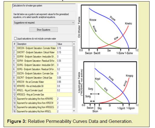
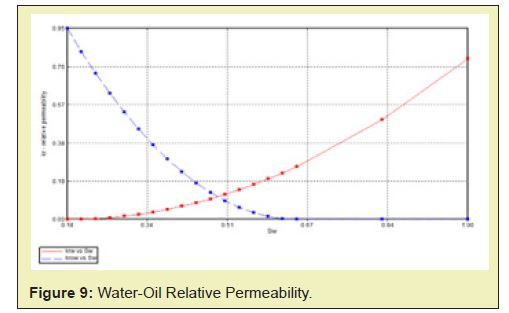
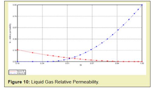
Defining rock-fluid properties

The first step under this section was to create or edit new rock type by generating tables using correlation. In the Relative Permeability Correlations window, the information presented in Figure 3 were inputted to define the Relative Permeability Curves as shown in in the same figure. Quadratic Smoothing was chosen for both the Water-Oil Table and the Liquid-Gas Table.

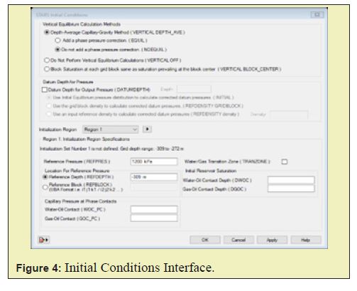
Defining initial conditions

This is the section where the reservoir reference pressure and the depth were specified, and the default of Depth-Average Capillary-Gravity Method for Vertical Equilibrium Calculations was used as shown in the Figure 4.

Defining numerical controls

This is the section where a value of 0.01day was used for the DTWELL and autotune was set ON.

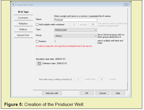
Defining wells and constraints

For the SAGD model, an injector well was placed above a producer well. Due to this, two wells were defined under this section. Well Newunder Wells and Recurrent section was clicked to first create a production well which was named producer and under “type”, PRODUCER was selected as shown in Figure 5.

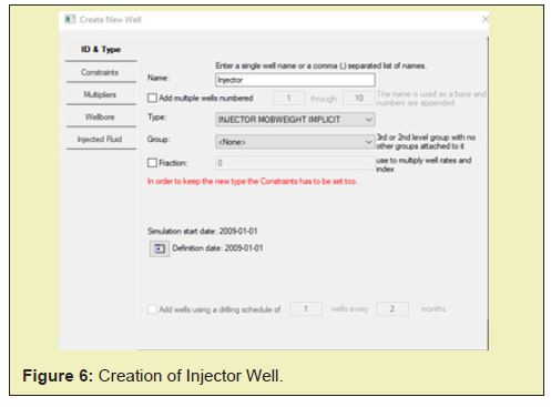
Another well was added in the same way and named as injector and under the “type”, INJECTOR MOBWEIGHT IMPLICIT selected as shown in the Figure 6.

After the wells were added, the well perforation needed to be defined before this section was complete. The well completion (PERF) window was opened under the Wells and Recurrent section. In this window under the General tab for the Injector well the Geometry Direction was changed to J-axis. The Well Radius was specified to 0.089m.

Artificial Intelligence

The Salford Predictive Modeller, a data mining and analytics platform that allows for the development of predictive, descriptive, and analytical models from databases of any size, complexity, or organization was used. The Multivariate Adaptive Regression Splines (MARS), Predictive Model and Treenet Gradient Boosting Machine were also used in this study. MARS is a multivariate non-parametric regression method that uses piecewise linear segments known as splines to match nonlinear relationships between predictor and response target variables automatically (piecewise polynomials).¹⁰ The MARS approach uses a set of independent explanatory variables to predict the values of continuous dependent variables. The mathematical form of MARS as expressed in Equation 1 describes the non-parametric interaction between the dependent variable (gas production rate) and the basis function (BF) terms as follows:¹¹

where GPR is the output variable of the gas production rate predicted by the MARS model, C_o is a constant (intercept), M is the number of basis function term, C_k is the vector of unknown coefficients of the k^th basis function (k = 1, 2, …, M), β_k denotes the basis function which model the interaction between two or more variables. X represents the reservoir parameter input variables.

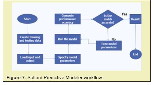
One of the most powerful strategies for developing predictive models is TreeNet Gradient Boosting. It is also the most versatile and powerful data mining tool on the market, capable of regularly producing highly accurate models. The precision of the TreeNet modelling engine is typically not achieved by single models or ensembles such as bagging or conventional boosting. CART is the most significant component of TreeNet gradient boosting and applications. Figure 7 shows the main procedure carried out in the modelling of the data.

Data entered in the Salford Predictive Modeler was the results obtained from CMG. The file format used was CSV (Comma Delimited). The accuracy of the model was computed using the R²(Equation 2) which is a statistical index having the characteristics of its optimum value closer to 1.0 as the best model prediction and Mean Absolute Percentage Error (MAPE) (Equation 3). The results obtained from Salford Predictive Modeler was then plotted in Microsoft Excel in combination with results from CMG for comparison.

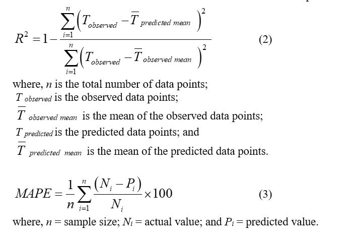
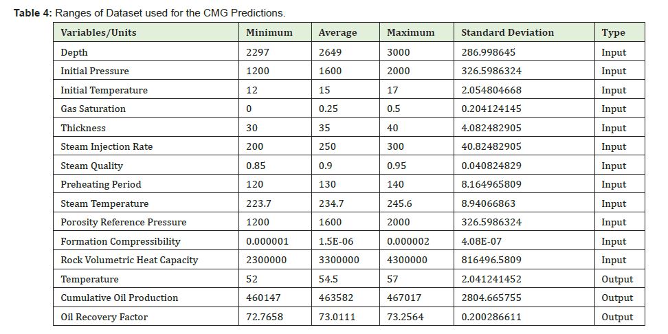
Table 4 shows the ranges of dataset that was used for the CMG results predictions using the Salfold Predictive Modeller.

The produced results include a three-dimensional reservoir model, a graph of cumulative oil production, oil recovery factor, water cut, cumulative steam oil ratio (CSOR), oil production rate against time and a plot of the sensitivity analysis of the bottomhole pressure and injector location on the oil recovery factor.

Reservoir model

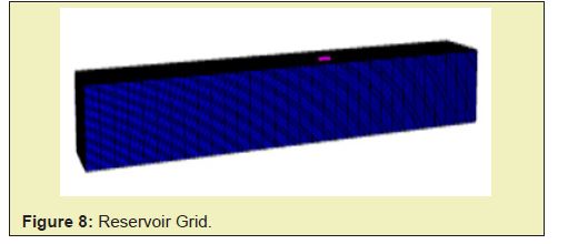
Figure 8 shows the developed reservoir grid in the i, j, and k direction. There were 111 blocks in the i-direction, 32 blocks in the j-direction, and 30 blocks in the k-direction in the reservoir grid.

Figures 9 and 10 show the water-oil and liquid-gas relative permeability curves, respectively. These relative permeability curves and residual fluid saturations were used to determine the oil production rate and ultimate recovery.

Sensitivity analysis

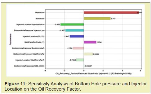
The Oil Recovery Factor Tornado Plot is presented in Figure 11. All of the experiments' maximum and minimum objective function values are shown by the maximum and minimum bars. Parameters with higher values on the plot are more sensitive to value changes than parameters with a low value. The injector location parameter was the most sensitive (changing this parameter’s value causes a negative effect on oil recovery factor of 2.422 bbl). In contrast, the injector location well pairs per pad and bottomhole pressure values did not have much effect.

Oil viscosity distribution

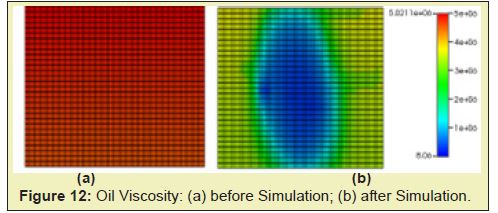
The Figure 12 shows the distribution of the oil viscosity before and after simulation of the reservoir. Figure 12 (a) indicates how high the reservoirs viscosity was at the start of the process. However, after the injection of steam and methane into the reservoir the reservoir viscosity reduced tremendously as can be seen in Figure 12 (b).

Effects of temperature on oil recovery factor

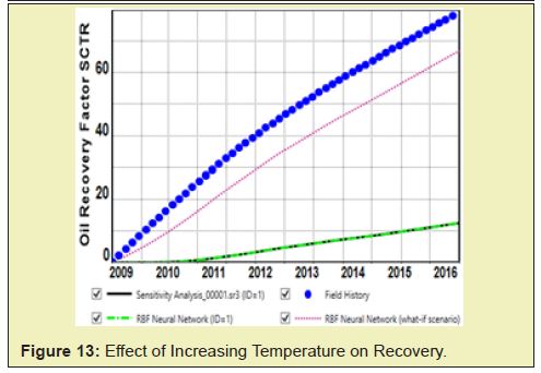
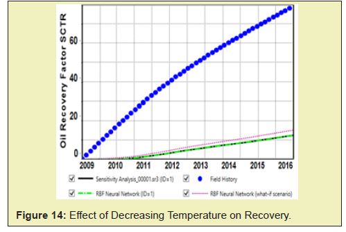
Figures 13 and 14 show the effect of temperature on the oil recovery factor. As temperature increase the viscosity of the oil reduces and as a result increase the oil mobility leading to a higher oil recovery as depicted in Figure 13. A decrease in temperature also result in a reduction of the oil viscosity leading to a low oil recovery factor as shown in Figure 14.

Oil recovery factor (rf) analysis

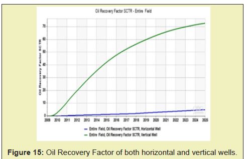
Figure 15 shows the resulting recovery factors (RF) obtained for both the vertical and horizontal wells. The data from the vertical well yielded the lowest recovery, whereas the data from the horizontal well yielded the highest. The overall improvement in recovery is inconsistent in both cases. Drilling horizontally, parallel to the geologic layers in tight formations, helps producers to access more of the oil- and natural gas-bearing rock than drilling vertically, with an approximate RF of 75%. Horizontal wells' lateral length increased, providing for more exposure to oil- and gas-producing geology from a single well.

Cumulative oil production analysis

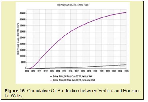
The cumulative oil production result is presented in Figure 16. The horizontal well gave the higher cumulative oil produced as compared to the vertical well. The cumulative oil from the vertical well was very low at the beginning of production but started to increase gradually till the end of production, even though the increase was not rapid as compared to the horizontal well.

Analysis of cumulative steam oil ratio

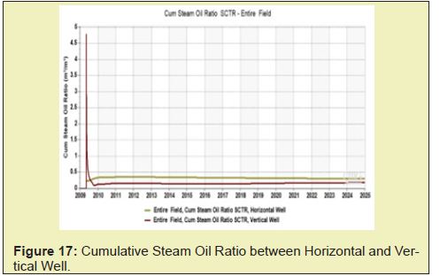
From Figure 17 the vertical well was observed to hold the highest CSOR at the beginning of production (2009) and started to decrease from the beginning of 2010 throughout to 2025 (end of production). The horizontal well on the other hand had CSOR values greater than the vertical well from the beginning of the production, particularly year 2010 to the end. Cumulatively, the horizontal well had the highest CSOR as compared to the vertical well.

Oil rate, SC analysis

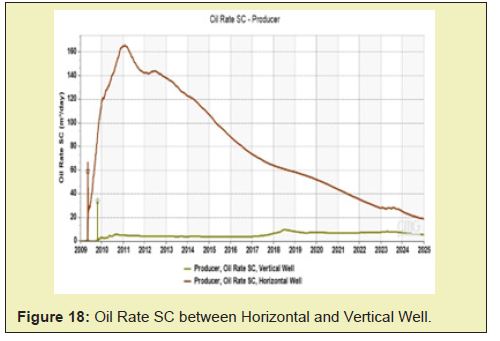
Figure 18 shows the oil rate for both the horizontal and vertical wells. The data obtained from the horizontal well seemingly has the highest rate (165m³/day) from 2009 to 2014 when it started declining gradually. Then it started to increase from 2023 and decreased again till 2025 (end of production) where the reservoir reached its economic limit. Following 2014, all the rates began to fall at the same pace. The viscosity data acquired from the vertical well has the lowest rate throughout this time period. Vertical well appears to have the lowest rate until 2018, when it began to gradually climb and then remained constant until 2025.

Water cut analysis

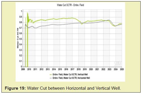
Generally, oil production decreased with increasing water and gas production. As shown in Figure 19, the horizontal well which gave the higher oil recovery increase in water production from the beginning of the production but plateaued and later reduced at 2024 where both the vertical and the horizontal became the same (which means the well has reached its economic limits). Wells preferentially producing water led to lower oil recovery rates, and this is evident in the vertical well. It can therefore be stated that the well position influences oil production, water cuts and ultimately oil recovery factors.

Results validation

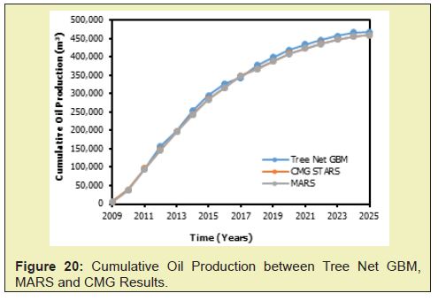
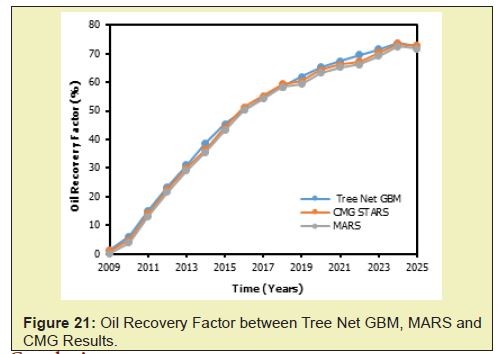
Results from the validation of predictions from CMG, MARS and Treenet GBM using SAGD model are presented in this section. Figures 20 and 21 show the validation on cumulative oil production and oil recovery factor from the three methods, respectively. The results showed perfect match between the methods with the Mean Absolute Percentage Errors (MAPE) and coefficient of regressions (R²) presented in Tables 5 and 6.

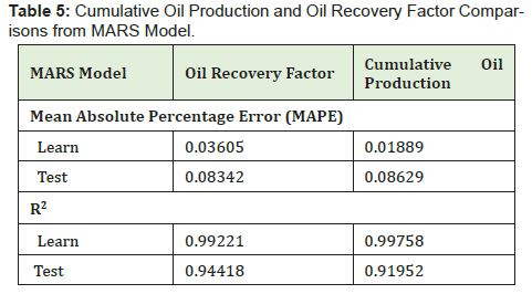
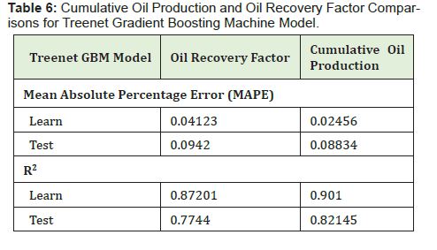
In this study, a layered heterogeneous reservoir model was built using CMG simulator to study a SAGD process of which different reservoir parameters were considered. Based on the results accumulated from this study, the horizontal well gave a higher oil recovery factor than the vertical well and based on that, the horizontal well is more preferred. The MARS offered better accuracy in the determination of cumulative oil production (R²=0.99758; MAPE=0.01889) and oil recovery factor (R²=0.99221; MAPE=0.03605) when compared to the Treenet GBM machine learning technique by recording lower MAPEs and higher R² values.

The authors acknowledge University of Mines and Technology for their support in terms of computer facility to produce this paper.

None.

Authors declares that there is no conflicts of interest.

1. 1. Færgestad IM. Heavy oil, Oilfield Review. 2016.
2. 2. Zhouyuan Z. Efficient Simulation of Thermal Enhanced Oil Recovery Processes, Unpublished PhD. Thesis, Stanford University, California, USA. 2011:pp.237.
3. 3. Marianayagam KR. Numerical Simulation Study on Parameters related to Athabasca Bitumen Recovery with SAGD, Unpublished MSc. Project Work, Norwegian University of Science and Technology, Trondheim, Norway. 2012:pp.122.
4. 4. Santos R, Loh W, Bannwart A, et al. An Overview of Heavy Oil Properties and Its Recovery and Transportation Methods. Brazilian Journal of Chemical Engineering. 2014;31(3):571–590.
5. 5. Energy Education. Energy Education-Steam Assisted Gravity Drainage. 2018.
6. 6. Zargar Z, Razavi SM, Ali SF. Analytical model of steam-assisted gravity drainage (SAGD) process in relation to constant injection rate. Fuel. 265:116772.
7. 7. Fayazi A. Kantzas A. A Review on Steam-Solvent Processes for Enhanced Heavy Oil/Bitumen Recovery. Reviews in Chemical Engineering. 2019;35(3):393–419.
8. 8. Speight JG. Enhanced Recovery Methods for Heavy Oil and Tar Sands. Gulf Publishing Company. 2009: pp.354.
9. 9. Anon. “SAGD Simulation using STARS”. Unpublished Company Manual, CMG. 2020:pp.57.
10. 10. Brantson ET, Binshan J, Busayo OO. Development of Machine Learning Predictive Models for History Matching Tight Gas Carbonate Reservoir Production Profiles. Journal of Geophysics and Engineering. 2018;15:2235–2251.
11. 11. Friedman JH. Multivariate Adaptive Regression Splines. The Annals of Statistics. 1991:pp.1–67.