Trends in Petroleum Engineering

Unconventional resources have emerged as one of the crucial alternatives to the rapidly depleting of conventional hydrocarbon resources. The hydrocarbon potential of shale source rocks is assessed by the percentage of the organic index such as total organic carbon (TOC). Correct estimation of TOC is very important since minor deviations in anticipated results can lead to wastage of investments and time. A slight improvement in estimation practices, on the other hand, can increase the value of an exploration project. Therefore, the objective of this study is to present an improved classification and regression tree (CART) computational learning-based model as an improved alternative in estimating TOC from well logging data. Conventional well logs suite of bulk density, gamma-ray, deep resistivity, sonic transit time, spontaneous potential, and neutron porosity from Mihambia, Mbuo and, Nondwa, Formations of the Mandawa Basin Tanzania, were used as input variables. Results from the developed CART TOC model were compared with the random forest (RF) and backpropagation neural network (BPNN). It was observed that the proposed CART model trained better while generalizing better through unused testing data compared with RF and BPNN. CART model achieved R, RMSE, and MAPE values of 0.9615, 0.0840, and 0.5035 for training and 0.9703, 0.1162, and 0.3722 for testing respectively. The proposed model work with higher accuracy with the sensitivity analysis indicating that gamma-ray, deep resistivity, and sonic transit time significantly influenced the model outcome.

Keywords: Total organic carbon, Classification and regression tree (CART), Machine learning, Well logging

As global oil and gas consumption is upswing and conventional oil reserves are diminishing, the world's huge discovered shale resources have recently drawn much more attention. Such an unconventional resource has emerged as one of the most essential substitutes to the rapid decrease of conventional resources. The exploration and exploitation of unconventional hydrocarbons resources such as shale oil and gas rely particularly on reliable and accurate evaluation of total organic carbon content (TOC). TOC is a measure of the amount of organic matter present in a rock sample.^1,2 Not only that TOC content exhibits the potential hydrocarbon-in-place and quality of the source rock, but also it offers important information about wettability, porosity, rock texture, permeability microstructure, and hydraulic fracturing design of the shale reservoirs.

The most accurate estimation of TOC content is the direct measurement of organic richness in the laboratory on the core samples or using rock-eval pyrolysis.³ On contrary, obtaining core samples from each well in the field and conducting laboratory tests on them is costly and a time-consuming approach. As a result, core-based data are scarce and expensive. In line with this well log data being a critical aspect of mostly well drilling designs are easily accessible. Therefore, to generate correlations that can be applied to the entire well with limited core sample data, related well logs are used.

Different researchers have highlighted the relationship between TOC and geophysical well logs.^4-8 The idea being focused on the reaction and response of well logs signals on the available organic matter. Therefore, the high response of acoustic, resistivity, and spectral gamma-ray, logs is directly proportional to the increase of TOC values. However, bulk density logs have an inverse proportional to the increase of TOC values. Using data from Devonian shale formation, Schmoker⁹ introduced and developed the density log-based technique. Schmoker’s technique is empirical and assumes that any change in bulk density is due to the presence of kerogen. Passey¹⁰ suggested a ΔlogR technique for identifying source rocks by overlaying porosity logs and resistivity logs. Nevertheless, this is an empirical method and was not developed from rock physics principles.¹¹ It's worth noting that, the nonlinear relationship between well logs and TOC in many shale rocks may highly reduce the estimation accuracy of TOC using both Schmoker’s and ΔlogR techniques.

The successful application of computational intelligence (CI) in hydrocarbon exploration and exploitation in recent years, has seen the adoption of intelligence learning models in predicting TOC from well log data.^12-23 Computing intelligence is a captivating discipline that combines computational power with human intelligence to develop sophisticated and trustworthy solutions to stunningly nonlinear and complicated problems. The CI models have the advantage of being able to adapt and learn to the dynamic conditions of the reservoir such as depositional and formation environment whilst utilizing the entire suite of well logs for better prediction of TOC.^24-27 A vast variety of studies indicate that correct utilizing these non-linear algorithms, the TOC content can always be predicted more accurately.^28-32 Artificial neural network (ANN) has been the most commonly utilized computational learning technique for predicting TOC in studies.^33-39 Compared to traditional approaches such as ΔlogR, an ANN performed excellently in these studies due to its capability to draw out patterns between the range of input well logs and measured TOC data. On the contrary constant tuning of the ANN parameters such as number of hidden nodes, biases, and weights to achieve the best performing model structure, ANN suffers intrinsic drawbacks such as overfitting, low computational speed, and converging at local minima.

It is important to address that numerous studies have recommended novel concepts and enhanced learning algorithms as a substitute to the standard ANN. The idea of an incorporated semi-supervised computational intelligence model was use to predict TOC accurately without the requirement for manual overlapping of log curves.⁴⁰ Tan⁴¹ used support vector regression (SVR) in predicting TOC content in a gas-bearing shale and achieving better results. The application of an extreme learning machine (ELM) in predicting TOC in a shale gas reservoir was also investigated.⁴² Mahmoud⁴³ employed the use of new artificial neural networks (ANN) to establish an empirical equation for TOC predictions from conventional well logs data. Self-adaptive differential evolution-artificial neural network (SaDE-ANN) model also showed high accuracy in predicting TOC based on well logs data.^21,44 Gaussian process regression (GPR) was also implemented to predict TOC.^45,46 However, in order to achieve the optimal estimation results of GPR, the user requires to specify the best kernel function. Similar to ELM, most of those computational learning models require an iterative tuning of parameters training to achieve the best performance.

Therefore, we proposed the applicability of classification and regression tree (CART) model to predict TOC using inputs from well log parameters. The CART algorithm is the tree-based technique with the advantage of not being prone to overfit and can perform excellently even when the predictive variables are irregular. The performance of the CART model was further compared with untested computational learning methods of random forest (RF) and backpropagation neural network (BPNN). The result of the present study will rank the CART algorithm to a fairly new computational learning TOC model as an intelligent approach for the reliable prediction of TOC values. The rest of this paper is organized as follows: Section 2 presents the geological setting and data processing. Section 3 introduced three different methods for TOC estimation: BPNN, RF, and CART. Section 4 shows the results and discussion. Section 5 is the conclusion.

Mandawa basin is located in southern coastal Tanzania, separated by Ruvuma saddle in the South and Rufiji River in the North Figure 1. The geological evolution of the Mandawa basin has been studied by different researchers.^47-49 Karoo rifting, Gondwana breakup, East African rift system and opening of Somali basin are the main factors controlled the evolution of Mandawa basin.^50-52 The Mandawa Basin's depositional history was mainly influenced by the Gondwana breakup. Mandawa, Kilwa, Pindiro, Songosongo and Mavuji are the main five groups that are found in the basin. Before the break-up of Gondwana, the depositional environment was continental with both deltaic and fluvial deposits dominating the area.⁵³ Followed by the development of rifting and drifting, restricted marine embayment with barrier reefs were formed from Paleo-Tethys transgression isolating several saline lagoons during the early to middle Jurassic.⁵⁴ In the late Jurassic the basin was subjected to rapid subsidence which last to the early Cretaceous leading to the deposition of clastic sediments in which the fluvial and alluvial deposits of the Mandawa and Mavuji groups were deposited. From the Aptian to the Paleogene, a mid-to-outer shelf zone of coastal Mandawa Basin was declined at a constant speed which resulted to the formation of Kilwa group.^55-63 The source rock of the Mandawa basin consists of Nondwa shales of the lower Jurassic Pindiro Group and Mbuo Claystone of the upper Triassic Pindiro Group.⁶⁴

The conventional well log data of neutron porosity (NPHI), gamma-ray (GR), spontaneous potential log (SP), deep lateral resistivity log (LLD), sonic travel time (DT), bulk density log (RHOB), and measured TOC values collected from Mandawa basin were used in this study Figure 2. Furthermore, 56 data points of TOC from two wells namely Mbate and Mbuo were used to train the intelligent models while 27 data points of TOC from the Mita Gamma well were used to test the validity of developed models. The statistical features for three different wells suite of Mita Gamma, Mbate, and Mbuo which were used to learn models developed are analyzed in Table 1.

During data processing, feature selection (variable selection) was performed to identify and delete obsolete, unnecessary, and redundant data attributes that do not add to a predictive model's accuracy or may minimize the model's accuracy. Pearson correlation coefficient (R) was used to evaluate the relative impact of the input variables on the output Equation 1. The correlation coefficient (R) values always lie in the range between 0 and 1. In this case, the values close to positive indicate a similar relationship between two separate variables, whereas near-zero values indicate a weak relationship between the two-variable pair, and near-negative values indicate an inverse relationship between independent variables.
,                                                                                (1)
where  represents the correlation coefficient of variables a and b,  and  are the standard deviations for variables a and b, respectively. Well log data and measured TOC were both normalized in the scale between 0 and 1 to reduce the redundancy as well as to improve the integrity of the data. The normalization processing was done using Equation 2:
                ,                                                                               (2)
where  represents the original value,  represents the normalized value of the dataset, is the maximum value and is the minimum value. The selected technique enables the computational learning algorithm to execute faster, improves the accuracy of the model, reduces the overfitting, and also it decreases the complexity of the model.⁶⁵ The relevance of the input data for predicting the TOC is shown in Figure 3.

The BPNN is a feedforward network which consists of many layers. These layers have been trained using the method of error backpropagation. BPNN comprises three types of layers: hidden, input and output layers.⁶⁶ For hidden and output layers, the neurons presented appear to contain biases, which link to units whose activation is always 1. The bias concept often works as a set of weights. Signals are sent in the opposite directions during the back-propagation learning phase. The BPNN is served as a way to solve the multi-layer perceptron training problem.⁶⁷ The internal network weight change after each training epoch due to backpropagation error and addition of differentiable function at each node, were the major advances for BPNN method.

The flow of data in BPNN is divided into two phases. In the first phase, the input data is displayed forward to the output layer from the input layer, which results in an actual output shown inEquation3.⁶⁶ The BPNN model can be presented by the following equation: ,                                                         (3)
where  represent the input vector dimension,  is the hidden neurons number, Y is the output variable and x stand for input variables. Note that  and  stands for bias weights. All of the connection weights (along with the bias weights) are initialized with small random numbers, and an iteration process is used to calculate the final values. The sigmoid activation function, f, is the most widely used and can be presented as in Equation 4:
 ,                                                                                (4)
For the second phase, the errors between the target and real values are disseminated backward from the output layer to the preceding layers and the connection weights are adjusted to reduce the errors between the actual and target output values. The overall error can be calculated by the total sum of errors (TTS) as shown in Equation 5.
           ,                                                               (5)
where T and C represent the target and calculated signals, respectively and  represent the total number of training pairs. BPNN algorithms, on the other hand, have weaknesses such as low iteration speeds and a greater tendency to collapse into local minimums. The algorithm used in this study was Levenberg-Marquardt (LM). The LM algorithm is a technique for determining the minimum of a multivariate function expressed as the number of squares of non-linear real-valued functions iteratively.^68,69 The Gauss-Newton and steepest descent method combines to for an algorithm of LM. When the current solution is not close to the correct solution, the algorithm effectively functions as a steepest descent method. When the current solution is close to the correct solution, the algorithm becomes the Gauss-Newton method. ⁷⁰

Random forest (RF)

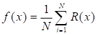
Random forest is the method of ensemble learning that is mostly used for regression, classification, and other tasks. During training, it is generally focused on developing multiple decision trees and giving out the classes or predicting each tree.⁷¹ Random Forest combines two methods of Bagging and Features Randomness which helps to get highly accurate results, avoid overfitting problems, and ability to handle larger input datasets and thus make it suitable for the prediction purpose. From the set of training data, the Bagging technique is often used to train each individual tree.⁷² To get a split at each node, this approach just looks at a random subset of variables. Each tree in random forest can only be selected from a random subset of features (Feature randomness). The increased diversification and lower correlation are the results of significant trees variation in the model. As a result, in a random forest, we finish up with trees that are not only trained on different sets of data but also make decisions based on the use of different features.⁷³ The general RF algorithm can be presented by Equation 6.
 ,                                                                               (6)
where R (x) represent the individual regression result tree (RT), f(x) is the RF result, and N represent number of trees.

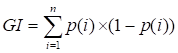
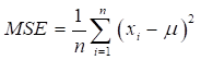
The benefit of the RF is that it can determine the relative importance of parameters, which can be obtained using two methods, Gini impurity (GI) and mean square error (MSE). The GI is used to estimate the quality of each division on each variable in a tree, and the MSE is used to determine the average decrease in prediction accuracy due to partition on each predictor.^71,74 The GI and MSE can be presented in Equations 7 and 8, respectively.
     ,                                                               (7)
   ,                                                               (8)
where p(i) represents the probability of randomly choosing an observation of class I, n represent the number of classes,  is the label for an instance and  is the mean given by Equation 9 below:
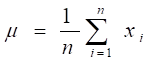,                                                                            (9)
The predictor variables of multiple types can leads to the unbalance of the GI approach.  The MSE (mean square error) approach was proposed to measure the relative importance accurately as compared to the GI method.75 As a result, the RMSE (random mean square error) approach was chosen to predict relative importance in this study. The Random Forest algorithm may include the following steps:

1. i. Random samples selection from given dataset.
2. ii. Decision tree construction for every sample. The forecast result from each decision tree will then be obtained.
3. iii. From every forecasted result, then the voting can be calculated.
4. iv. The final prediction output is obtained from the result of most voted prediction tree. The illustration of the working principle of the RF algorithm is shown in Figure 4.
Classification and Regression Tree (CART)

Classification and Regression Tree (CART) method was introduced to describe a decision tree approach which can be used to overcome the challenges arisen from the built predictive modeling of either classification or regression.⁷⁶ A nonparametric modeling technique by using group of independent categorical or continuous variables is employed to describe the dependent’s responses. CART generates a classification tree for categorical dependent variable and regression tree when dependent variable is continuous. The decision tree is the CART’s output with each fork indicating a split in a predictor variable and each end node containing an outcome variable prediction.⁷⁷ The most valuable characteristic of CART is the ability to process various kinds of datasets. On top of that, it can also handle a huge amount of data easily.⁷⁸ CART models are simple to learn and operate which giving them a significant advantage when compared to other analytical models.

The steps of building a CART model are mainly based on the following two steps. The first step is to develop the decision tree. CART's basic principle is to identify an optimal feature in the original dataset by improving through some criteria and splits. CART always chooses the feature with the lowest Gini information gain in the existing data set as the decision tree's node division. Basically, the sample sets to be categorized are separated into two sub-sample sets using the Gini index technique and cycled through this step until the present sample sets to be categorized are recognized to be leaf nodes or a requirement for terminating the classification is achieved. The decision tree is pruned in the second step. To build an optimal tree, the tree must be pruned to minimize overfitting. In general, the nodes of the tree must be pruned to manage the tree's complexity, which is determined by the number of leaves on the tree. Furthermore, a cross-validation approach is used to determine the best tree size.

The most often used criteria for splitting the trees are "Entropy" for the information gain and "Gini" for the Gini impurity, which can be represented mathematically as in Equation 10 and Equation 11.
      ,                                                                               (10)
      ,                                                                               (11)
where P is the probability of class i and k is the total number of classes.

CART models use variance minimization methods to iteratively divide data to determine progressively homogenous groups using independent variable splitting criteria. The dependent data is divided into a sequence of right and left leaf nodes that descend from root nodes as shown in the decision tree structure in Figure 5. The main weakness of this method is the risk of data over-fitting, which occurs when trees grown to their full size match the training data so well that they are unable to extrapolate effectively.⁷⁹

The statistical indicators used to judge the performance of the predictive models were correlation coefficient (R), root means square error (RMSE), and mean absolute percentage error (MAPE). R measures the strength and direction of the linear relationship between predicted and measured TOC variables, RMSE measures the relative average square of the errors and represents the stability or quality of the models while MAPE describes the model in terms of the percent accuracy. The mathematical expression for R, RMSE, and MAPE is given in Equations 12, 13, and 14.

  ,                                                               (12)
  ,                                                               (13)
     ,                                                               (14)
where  is the predicted TOC value from the models,  represents the actual TOC value measured from core samples,  and  are the mean values of the predicted and actual TOC, and n represent the number of samples.

During training, the uncertainty concerning the optimal CART and RF learning rate was solved using the widely used sequential trial and error method. The learning rate that generated the best TOC prediction for CART was observed at 0.12 with a maximum of 190 trees and the maximum nodes on each tree were specified at 13. Similarly, for RF the learning rate that generated the best TOC prediction was observed at 0.16 with a maximum of 200 trees and the maximum nodes on each tree were specified at 6. The tuning parameter in the architecture of BPNN was the number of hidden neurons which was also obtained as a result of the sequential trial and error method.

During training, it was identified that the CART TOC model trained better than both RF and BPNN. CART had RMSE, and MAPE values of 0.0840, and 0.5035 respectively as shown in Table 2. RF TOC model trained slightly worse with R, RMSE, and MAPE values of 0.9522, 0.0968, and 0.5915 respectively as seen in Figure 7. The TOC model that had the worst training performance was the BPNN with R, RMSE, and MAPE values of 0.9390, 0.1556, and 0.9053 Figure 6.

A good result for the CART TOC model was also observed for the case of the correlation coefficient. During training, CART obtained a high R-value of 0.9615 compared to 0.9522 and 0.9390 obtained by RF and BPNN respectively as seen in Figure 7. The observed scatter diagram correlates measured TOC values against the predicted TOC results from all trained models of CART, BPNN, and RF. The tight cloud of data points about the diagonal line for training data presents the good prediction accuracy of the TOC-developed models. The performance of the developed predictive CART, BPNN, and RF models during the training process is described as compared to the TOC measured data in Figure 8. The obtained results indicate that the CART TOC model has a greater ability to predict TOC with high accuracy as compared with RF and BPNN during training.

Here, unused 27 data points of TOC from the Mita Gamma well were used to test the validity of developed models. It was revealed that the CART TOC model was the best performing model which generated predictions close to the actual TOC values. Table 3 summarizes the results obtained during the validation process (testing). This was seen in Figure 9 as CART obtained the least RMSE and MAPE values of 0.1162 and 0.3722 respectively.

The least RMSE and MAPE score from CART indicates that the TOC predictions results do not deviate much from the measured TOC value. The extent of deviation from the measured TOC value can be examined visually from Figure 10. Therefore, the least RMSE value of 0.1162 during testing makes the proposed CART TOC model the best and most stable TOC model when compared to RF and BPNN. The RF TOC models produced prediction scores of 0.1383 and 0.3874 for RMSE and MAPE respectively. BPNN produced error margin or RMSE and MAPE as 0.5890 and 0.7272 respectively, this makes it a poor permed model. The R-value for CART was the highest score of 0.9703 as indicated in Table 3. Compared to RF and BPNN, the CART model can be described as the most resilient to outliers when dealing with noisy data. The RF and BPNN models scored 0.9449 and 0.9122 as R-values respectively Figure 11. Thus, the output from the statistical error analysis ranks CART as the best performing TOC model.

The variable significance for the well log inputs for prediction of TOC was determined by the influence of the variables’ mean relative produced by the regression tree of CART. Figure 12 shows the TOC regression tree model built from well logs variables. It further shows the contribution of each input well log in the prediction of TOC. CART model selected five well logs out of the six inputs as the most important variables for TOC prediction. The GR was the first important variable in predicting TOC with 45 fields of GR less than 0.63 and an average of 0.195. RHOB became the second important variable with 33 fields and it impacted those fields with high RHOB. The third important variable was SP with 30 fields and an average of 0.111 followed by DT with 17 fields and the last one was NPHI with 15 fields and an average of 0.067.

The present study proposed the predictive capability of the classification and regression tree (CART) model in predicting TOC from petrophysical well logs of the Mihambia, Mbuo, and Nondwa Formations in the Triassic to mid-Jurassic of the Mandawa Basin, southeast Tanzania. The models were trained using well log data from Mbuo and Mbate wells while the well logs data from Mita Gamma well were used to test the validity of the developed model. Based on this, input parameters of a well log suite of GR, SP, NPHI, DT, LLD, and RHOB, were used to develop the TOC models. The evaluation of the proposed model was based on various statistical measures such as RMSE, MAPE, and R.

The results from the experimental study by using both training data and testing data revealed that the CART model produced higher accuracy and correlation with core data when estimating TOC than BPNN and RF models. The variable significance analysis was used to identify the important contribution of the individual well log on the model performance. It was revealed that well logs parameters of GR, SP, DT, NPHI, and RHOB have greater contributions to the performance of the CART model in TOC prediction. This makes CART a more reliable CI technique for attaining accurate TOC estimation.

The authors acknowledge supports from National Natural Science Foundation of China: No. 51704265 (Research on two component gas diffusion-convection model in enhancing shale gas recovery with CO2 injection PI: Dr. Chaohua Guo), the Outstanding Talent Development Project of China University of Geosciences (CUG20170614), and the Fundamental Research Founds for National University, China University of Geosciences (Wuhan) (1810491A07).

None.

The author declares that no conflict of Interest.

1. 1. Zongying Z. Quantitative analysis of variation of organic carbon mass and content in source rock during evolution process. Petroleum Exploration and Development. 2009;36(4):463-468.
2. 2. King GE. Thirty Years of Gas Shale Fracturing: What Have We Learned?, SPE Annual Technical Conference and Exhibition. 2010.
3. 3. Xiong H, Wu X, Fu J. Determination of Total Organic Carbon for Organic Rich Shale Reservoirs by Means of Cores and Logs, SPE Annual Technical Conference and Exhibition, 2019, Society of Petroleum Engineers. 2019.
4. 4. Asante Okyere S, Ziggah YY, Marfo SA. Improved total organic carbon convolutional neural network model based on mineralogy and geophysical well log data. Unconventional Resources. 2021;1:1-8.
5. 5. Amosu A, Imsalem M, Sun Y. Effective machine learning identification of TOC-rich zones in the Eagle Ford Shale. Journal of Applied Geophysics. 2021;188:104311.
6. 6. Omran AA, Alareeq NM. Joint geophysical and geochemical evaluation of source rocks – A case study in Sayun-Masila basin, Yemen. Egyptian Journal of Petroleum. 2018;27(4):997-1012.
7. 7. Wang P, Peng S, He T. A novel approach to total organic carbon content prediction in shale gas reservoirs with well logs data, Tonghua Basin, China. Journal of Natural Gas Science and Engineering. 2018;55:1-15.
8. 8. Amiri Bakhtiar H, Telmadarreie A, Shayesteh M, et al. Estimating total organic carbon content and source rock evaluation, applying ΔlogR and neural network methods: Ahwaz and Marun oilfields, SW of Iran. 2011;29(16):1691-1704.
9. 9. Schmoker JWJAB. Organic content of Devonian shale in western Appalachian Basin. American Association of Petroleum Geologists Bulletin. 1980;64(12):2156-2165.
10. 10. Passey Q, Creaney S, Kulla J, et al. A practical model for organic richness from porosity and resistivity logs. AAPG Bulletin. 1990;74(12):1777-1794.
11. 11. Heidari Z, Torres Verdín C. Inversion-based method for estimating total organic carbon and porosity and for diagnosing mineral constituents from multiple well logs in shale-gas formations. Interpretation. 2013;1(1):T113-T123.
12. 12. Ahangari D, Daneshfar R, Zakeri M, et al. On the prediction of geochemical parameters (TOC, S1 and S2) by considering well log parameters using ANFIS and LSSVM strategies. Petroleum. 2021;8(2):174-184.
13. 13. Bai Y, Tan M. Dynamic committee machine with fuzzy-c-means clustering for total organic carbon content prediction from wireline logs. Computers & Geosciences. 2021;146:104626.
14. 14. Handhal AM, Al Abadi AM, Chafeet HE. et al. Prediction of total organic carbon at Rumaila oil field, Southern Iraq using conventional well logs and machine learning algorithms. Marine and Petroleum Geology. 2020;116:104347.
15. 15. Khoshnoodkia M, Mohseni H, Rahmani O, et al. TOC determination of Gadvan Formation in South Pars Gas field, using artificial intelligent systems and geochemical data. Journal of Petroleum Science and Engineering. 2011;78(1):119-130.
16. 16. Mulashani AK, Shen C, Asante Okyere S, et al. Group Method of Data Handling (GMDH) Neural Network for Estimating Total Organic Carbon (TOC) and Hydrocarbon Potential Distribution (S1, S2) Using Well Logs. Natural Resources Research. 2021;30(5):3605-3622.
17. 17. Rong J, Zheng Z, Luo X, et al. Machine Learning Method for TOC Prediction: Taking Wufeng and Longmaxi Shales in the Sichuan Basin, Southwest China as an Example. Geofluids. 2021;6794213.
18. 18. Sfidari E, Kadkhodaie Ilkhchi A, Najjari S. Engineering, Comparison of intelligent and statistical clustering approaches to predicting total organic carbon using intelligent systems. Journal of Petroleum Science and Engineering. 2012;86:190-205.
19. 19. Siddig O, Ibrahim AF, Elkatatny S. Application of Various Machine Learning Techniques in Predicting Total Organic Carbon from Well Logs. Computational Intelligence and Neuroscience. 2021;7390055.
20. 20. Zheng D, Wu S, Hou M. Fully connected deep network: An improved method to predict TOC of shale reservoirs from well logs. Marine and Petroleum Geology. 2021;132:105205.
21. 21. Elkatatny S. A Self-Adaptive Artificial Neural Network Technique to Predict Total Organic Carbon (TOC) Based on Well Logs. Arabian Journal for Science and Engineering. 2019;44(6):6127-6137.
22. 22. Shalaby MR, Jumat N, Lai D, et al. Integrated TOC prediction and source rock characterization using machine learning, well logs and geochemical analysis: Case study from the Jurassic source rocks in Shams Field, NW Desert, Egypt. Journal of Petroleum Science and Engineering. 2019;176:369-380.
23. 23. Tenaglia M, Eberli GP, Weger RJ, et al. Total organic carbon quantification from wireline logging techniques: A case study in the Vaca Muerta Formation, Argentina. Journal of Petroleum Science and Engineering. 2020;194:107489.
24. 24. Vikara D, Remson D, Khanna V. Machine learning-informed ensemble framework for evaluating shale gas production potential: Case study in the Marcellus Shale. Journal of Natural Gas Science and Engineering. 2020;84:103679.
25. 25. Zeng B, Li M, Zhu J, et al. Selective methods of TOC content estimation for organic-rich interbedded mudstone source rocks. Journal of Natural Gas Science and Engineering. 2021;93:104064.
26. 26. Menezes R. Using machine learning to predict total organic content–case study: Canning Basin, Western Australia. ASEG Extended Abstracts. 2019;2019(1):1-3.
27. 27. Tahmasebi P, Javadpour F, Sahimi M. Data mining and machine learning for identifying sweet spots in shale reservoirs. Expert Systems with Applications. 2017;88:435-447.
28. 28. Shalaby MR, Malik OA, Lai D, et al. Thermal maturity and TOC prediction using machine learning techniques: case study from the Cretaceous–Paleocene source rock, Taranaki Basin, New Zealand. Journal of Petroleum Exploration and Production Technology. 2020;10(6):2175-2193.
29. 29. Zhao P, Ostadhassan M, Shen B, et al. Estimating thermal maturity of organic-rich shale from well logs: Case studies of two shale plays. Fuel. 2019;235:1195-1206.
30. 30. Zhu L, Zhang C, Zhang C, et al. Prediction of total organic carbon content in shale reservoir based on a new integrated hybrid neural network and conventional well logging curves. Journal of Geophysics and Engineering. 2018;15(3):1050-1061.
31. 31. Pan W, Suping P, Wenfeng D, et al. Relationship between organic carbon content of shale gas reservoir and logging parameters and its prediction model. Journal of China Coal Society. 2015;40(2):247-253.
32. 32. Ouadfeul SA, Aliouane L. Total Organic Carbon Prediction in Shale Gas Reservoirs from Well Logs Data Using the Multilayer Perceptron Neural Network with Levenberg Marquardt Training Algorithm: Application to Barnett Shale. Arabian Journal for Science and Engineering. 2015;40(11):3345-3349.
33. 33. Chan SA, Hassan AM, Usman M, et al. Total organic carbon (TOC) quantification using artificial neural networks: Improved prediction by leveraging XRF data. Journal of Petroleum Science and Engineering. 2021;109302.
34. 34. Johnson LM, Rezaee R, Kadkhodaie A, et al. Geochemical property modelling of a potential shale reservoir in the Canning Basin (Western Australia), using Artificial Neural Networks and geostatistical tools. Computers & Geosciences. 2018;120:73-81.
35. 35. Alizadeh B, Najjari S, Kadkhodaie Ilkhchi A. Artificial neural network modeling and cluster analysis for organic facies and burial history estimation using well log data: A case study of the South Pars Gas Field, Persian Gulf, Iran. Computers & Geosciences. 2012;45:261-269.
36. 36. Barham A, Ismail MS, Hermana M, et al. Predicting the maturity and organic richness using artificial neural networks (ANNs): A case study of Montney Formation, NE British Columbia, Canada. Alexandria Engineering Journal. 2021;60(3):3253-3264.
37. 37. Bolandi V, Kadkhodaie Ilkhchi A, Alizadeh B, et al. Source rock characterization of the Albian Kazhdumi formation by integrating well logs and geochemical data in the Azadegan oilfield, Abadan plain, SW Iran. Journal of Petroleum Science and Engineering. 2015;133:167-176.
38. 38. Siddig O, Abdulhamid Mahmoud A, Elkatatny S, et al. Utilization of Artificial Neural Network in Predicting the Total Organic Carbon in Devonian Shale Using the Conventional Well Logs and the Spectral Gamma Ray. Computational Intelligence and Neuroscience. 2021;2486046.
39. 39. Tariq Z, Mahmoud M, Abouelresh M, et al. Data-Driven Approaches to Predict Thermal Maturity Indices of Organic Matter Using Artificial Neural Networks. ACS Omega. 2020;5(40):26169-26181.
40. 40. Zhu L, Zhang C, Zhang C, et al. A new and reliable dual model- and data-driven TOC prediction concept: A TOC logging evaluation method using multiple overlapping methods integrated with semi-supervised deep learning. Journal of Petroleum Science and Engineering. 2020;188:106944.
41. 41. Tan M, Song X, Yang X, et al. Support-vector-regression machine technology for total organic carbon content prediction from wireline logs in organic shale: A comparative study. Journal of Natural Gas Science and Engineering. 2015;26:792-802.
42. 42. Shi X, Wang J, Liu G, et al. Application of extreme learning machine and neural networks in total organic carbon content prediction in organic shale with wire line logs. Journal of Natural Gas Science and Engineering. 2016;33:687-702.
43. 43. Mahmoud AAA, Elkatatny S, Mahmoud M, et al. Determination of the total organic carbon (TOC) based on conventional well logs using artificial neural network. International Journal of Coal Geology. 2017;179:72-80.
44. 44. Sultan A. New Artificial Neural Network Model for Predicting the TOC from Well Logs. In SPE Middle East Oil and Gas Show and Conference, Society of Petroleum Engineers: Manama, Bahrain. 2019: p.13.
45. 45. Yu H, Rezaee R, Wang Z, et al. A new method for TOC estimation in tight shale gas reservoirs. International Journal of Coal Geology. 2017;179:269-277.
46. 46. Rui J, Zhang H, Ren Q, et al. TOC content prediction based on a combined Gaussian process regression model. Marine and Petroleum Geology. 2020;118:104429.
47. 47. Geiger M, Clark DN, Mette W. Reappraisal of the timing of the breakup of Gondwana based on sedimentological and seismic evidence from the Morondava Basin, Madagascar. Journal of African Earth Sciences. 2004;38(4):363-381.
48. 48. Nicholas CJ, Pearson PN, McMillan IK, et al. Structural evolution of southern coastal Tanzania since the Jurassic. Journal of African Earth Sciences. 2007;48(4):273-297.
49. 49. Fossum K, Dypvik H, Haid MHM, et al. Late Jurassic and Early Cretaceous sedimentation in the Mandawa Basin, coastal Tanzania. Journal of African Earth Sciences. 2021;174:104013.
50. 50. Hudson W. The geological evolution of the petroleum prospective Mandawa Basin southern coastal Tanzania. Trinity College Dublin, 2011.
51. 51. Kapilima S. Tectonic and sedimentary evolution of the coastal basin of Tanzania during the Mesozoic times. Tanzania Journal of Science. 2003;29(1):1-16.
52. 52. Reeves CV. The development of the East African margin during Jurassic and Lower Cretaceous times: a perspective from global tectonics. Petroleum Geoscience. 2018;24(1):41-56.
53. 53. Mtabazi EG, Boniface N, Andresen A. Geochronological characterization of a transition zone between the Mozambique Belt and Unango-Marrupa Complex in SE Tanzania. Precambrian Research. 2019;321:134-153.
54. 54. Salman G, Abdula I. Development of the Mozambique and Ruvuma sedimentary basins, offshore Mozambique. Sedimentary Geology. 1995;96(1):7-41.
55. 55. Bown PR, Jones TD, Lees J, et al. A Paleogene calcareous microfossil Konservat-Lagerstatte from the Kilwa Group of coastal Tanzania. GSA Bulletin. 2008;120(1-2):3-12.
56. 56. Godfray G, Seetharamaiah J, Geochemical and well logs evaluation of the Triassic source rocks of the Mandawa basin, SE Tanzania: Implication on richness and hydrocarbon generation potential. Journal of African Earth Sciences. 2019;153:9-16.
57. 57. Nicholas CJ, Pearson PN, Bown PR, et al. Stratigraphy and sedimentology of the Upper Cretaceous to Paleogene Kilwa Group, southern coastal Tanzania. Journal of African Earth Sciences. 2006;45(4):431-466.
58. 58. Hudson WE, Nicholas CJ. The Pindiro Group (Triassic to Early Jurassic Mandawa Basin, southern coastal Tanzania): Definition, palaeoenvironment, and stratigraphy. Journal of African Earth Sciences. 2014;92:55-67.
59. 59. Fossum K, Morton AC, Dypvik H, et al. Integrated heavy mineral study of Jurassic to Paleogene sandstones in the Mandawa Basin, Tanzania: Sediment provenance and source-to-sink relations. Journal of African Earth Sciences. 2019;150:546-565.
60. 60. Zhou Z, Tao Y, Li S, et al. Hydrocarbon potential in the key basins in the East Coast of Africa. Petroleum Exploration and Development. 2013;40(5):582-591.
61. 61. Smelror M, Fossum K, Dypvik H, et al. Late Jurassic–Early Cretaceous palynostratigraphy of the onshore Mandawa Basin, southeastern Tanzania. Review of Palaeobotany and Palynology. 2018;258:248-255.
62. 62. Berrocoso ÁJ, Huber BT, MacLeod KG, et al. The Lindi Formation (upper Albian–Coniacian) and Tanzania Drilling Project Sites 36–40 (Lower Cretaceous to Paleogene): Lithostratigraphy, biostratigraphy and chemostratigraphy. Journal of African Earth Sciences. 2015;101:282-308.
63. 63. Abay TB, Fossum K, Karlsen DA, et al. Petroleum geochemical aspects of the Mandawa Basin, coastal Tanzania: the origin of migrated oil occurring today as partly biodegraded bitumen. Petroleum Geoscience. 2021;27(1):2019-050.
64. 64. Maganza NE. Petroleum System Modelling of Onshore Mandawa Basin-Southern, Tanzania. Institutt for geovitenskap og petroleum. 2014.
65. 65. Al Abadi AM, Handhal AM, Al-Ginamy MA. Evaluating the Dibdibba Aquifer Productivity at the Karbala–Najaf Plateau (Central Iraq) Using GIS-Based Tree Machine Learning Algorithms. Natural Resources Research. 2020;29(3):1989-2009.
66. 66. Wang H, Wu W, Chen T, et al. An improved neural network for TOC, S1 and S2 estimation based on conventional well logs. Journal of Petroleum Science and Engineering. 2019;176:664-678.
67. 67. Rumelhart DE, Hinton GE, Williams RJ. Learning representations by back-propagating errors. Nature. 1986;323(6088):533-536.
68. 68. Marquardt DW. An algorithm for least-squares estimation of nonlinear parameters. 1963;11(2):431-441.
69. 69. Levenberg KJQoam. A method for the solution of certain non-linear problems in least squares. Journal of the Society for Industrial and Applied Mathematics. 1944;2(2):164-168.
70. 70. Gavin HP. The Levenberg-Marquardt algorithm for nonlinear least squares curve-fitting problems. Mathematics. 2013, 1-19.
71. 71. Breiman LJ. Random forests. Machine Learning. 2001;45(1):5-32.
72. 72. Breiman LJ. Using iterated bagging to debias regressions. Machine Learning. 2001;45(3):261-277.
73. 73. Peters J, De Baets B, Verhoest NE, et al. Random forests as a tool for ecohydrological distribution modelling. Ecological Modelling. 2007;207(2-4):304-318.
74. 74. Ouedraogo I, Defourny P, Vanclooster M. Application of random forest regression and comparison of its performance to multiple linear regression in modeling groundwater nitrate concentration at the African continent scale. Hydrogeology Journal. 2019;27(3):1081-1098.
75. 75. Genuer R, Poggi JM, Tuleau Malot C. Variable selection using random forests. Pattern Recognition Letters. 2010;31(14):2225-2236.
76. 76. Breiman L, Friedman J, Olshen R, et al. Classification and Regression Trees. 1984.
77. 77. Rokach L, Maimon O. Data Mining With Decision Trees: Theory and Applications. In World Scientific Publishing Co. Inc. 2014.
78. 78. Zekić-Sušac M, Has A, Knežević M. Predicting energy cost of public buildings by artificial neural networks, CART, and random forest. Neurocomputing. 2021;439:223-233.
79. 79. Bramer M. Principles of Data Mining. Springer Publishing Company, Incorporated: 2013.